What the benchmark threw away: classifying variable stars without their periods
Draw a star's light curve as a picture and an off-the-shelf ImageNet network will classify it about as well as the best time-series methods. Then every strong model we ran stalls at the same wall, the same kind of star read the wrong way. We find out what those stars have in common, rebuild the benchmark from OGLE-IV with the information it discarded, and measure what that information is worth.

Abstract
StarLightCurves is a standard time-series benchmark of 9,236 folded light curves: Cepheids, eclipsing binaries and RR Lyrae stars from the OGLE survey. We drew each curve as a picture in six ways and fine-tuned ImageNet networks on the pictures, using a fixed recipe and the same splits as the published time-series results. The best picture models reach 98.20%: level with MiniROCKET on the same splits (98.22%) and with HIVE-COTE 2 (98.19%, 30 published resamples), but not clearly above either. Pretraining is what makes them competitive: the same network trained from scratch scores 97.21%, and with only 25 training curves 87.40% against 96.84% with ImageNet weights.
Every strong model we ran then stalls at the same wall: 98% or more of the remaining errors are Cepheids and RR Lyrae mistaken for each other. The benchmark's own source paper calls their shapes "very similar" and says experts turn to other data. The benchmark doesn't store the number they usually turn to: the period. We rebuilt the dataset from OGLE-IV with periods kept (OGLE-SLC: same size, class mix and format). There, shape alone scores 99.10%, period alone 81.07%, and both together 99.40%, removing a third of the errors. The Cepheids still misread are mostly first-overtone Cepheids that pulsate faster than once a day. In period and in shape, they really are RR Lyrae look-alikes.
Why a navigator sorts stars
A pulsating star is a lighthouse with a known wattage. Classical Cepheids obey a period–luminosity relation: measure how long one takes to brighten and fade, and you know how bright it really is, so its apparent brightness gives its distance. That relation is "at the basis of the extra-galactic distance ladder".17 RR Lyrae stars do the same job closer in, with distance errors around 5%.18 Eclipsing binaries are something else entirely: two stars passing in front of each other. Their dips say nothing about how bright the system really is.
So the first question to ask of any variable star in a reference catalogue is which kind is it? Put an RR Lyrae on the Cepheid relation and, by our own arithmetic, its distance comes out badly wrong. At survey scale the question is asked by software: Gaia DR3 alone identified 10.5 million variable objects,19 and the Rubin Observatory, which began its ten-year survey on 29 June 2026, can issue up to seven million alerts a night.20 In 2023 one of us sketched an approach that has since become popular: turn light curves into images and let a vision model sort them. This note is the careful version of that experiment, and what it turned up.
The benchmark and what it dropped
StarLightCurves is one of the 128 datasets in the UCR time-series classification archive. Its light curves come from the OGLE-II survey of the Magellanic Clouds: 1,329 Cepheids, 2,580 eclipsing binaries and 5,327 RR Lyrae, matching the OGLE rows of the catalogue in Protopapas et al. (2006).1 Each star's photometry was folded on its period, so the x-axis is phase from 0 to 1, not time. It was then cleaned of spikes, smoothed, interpolated onto an even grid, aligned in phase by an approximate "universal phasing" step, and z-normalised.1,2 The archive's version has 1,024 points per curve, a fixed split of 1,000 training and 8,236 test curves, and unnamed labels 1, 2 and 3. Matching the class counts shows they are Cepheid, eclipsing binary and RR Lyrae.
Two things are gone from every curve. Z-normalisation removes the amplitude. Folding removes the period: the number used to fold each curve isn't stored anywhere in the files. For these three classes it is, as we show below, the most useful single number. The authors of the source paper said as much:
"despite CEPH and RRL being distinct star classes, the shapes of their light-curves are very similar … Indeed, domain experts resort to other data sources to classify CEPH and RRL light-curves correctly."
Rebbapragada et al. 2009, the paper the UCR archive lists as the dataset's source2
Even the phase alignment is approximate. The archive's description of the dataset,15 copied from a 2012 paper by the group that maintains the archive, calls the curves "(purportedly) phase-aligned", and notes that clustering improved sharply once rotations were allowed.3
Turning a curve into a picture
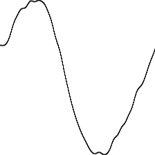
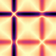
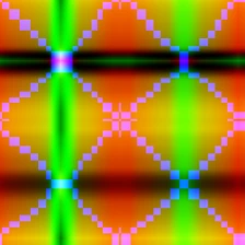
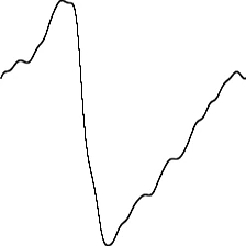
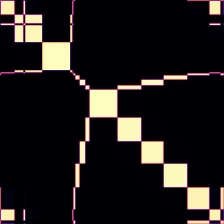
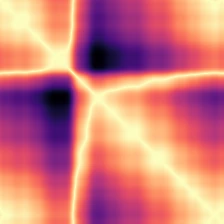
Image networks pretrained on ImageNet's photographs are free, mature and fast to fine-tune. To use one on a time series you have to draw the series first. We used six images: five drawings and a stack of three of them, all computed on the GPU from the raw series at 224 × 224 (Figure 1).
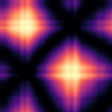
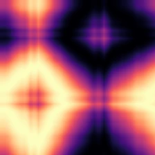

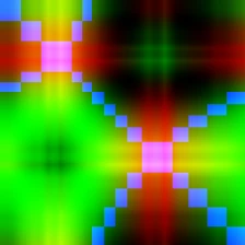
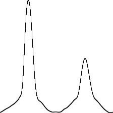
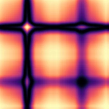
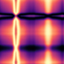
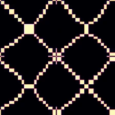
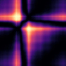
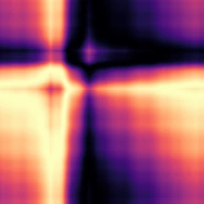
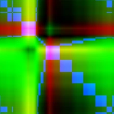
Gramian angular fields (Wang & Oates 2015).4 Shrink the series to 224 points by averaging windows (PAA), rescale to [−1, 1], and treat each value as the cosine of an angle, φi = arccos x̃i. Every pair of time points then becomes one pixel:
The summation field's diagonal is cos 2φi = 2x̃i2 − 1, which keeps each value's size but not its sign (it would keep both under [0, 1] scaling). The difference field's diagonal is zero.
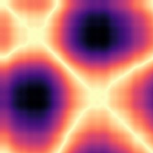
Markov transition field (also Wang & Oates).4 Sort the values into Q = 8 quantile bins, count how often the series steps from bin q to bin r to get a transition matrix W, and set pixel (i, j) to W evaluated at the bins of points i and j, computed at full resolution and block-averaged to 224 × 224. It keeps which level the curve is at, but only as one of eight bins, and summarises its movement as transition counts.
Recurrence plot. Pixel (i, j) is the distance |x̃i − x̃j|, left unthresholded. Eckmann et al. (1987) introduced the thresholded, delay-embedded original.5 Timage (2019) used this form with ImageNet ResNets.6
Line plot, the curve simply drawn as an anti-aliased line, and the stack,
GASF, GADF and MTF as the three colour channels, as Wang & Oates suggest.4 All six are
in lcdata.py, checked against direct NumPy implementations by test_encodings.py.
This idea isn't new on this dataset. Timage fine-tuned an ImageNet ResNet-50 on recurrence plots of StarLightCurves and reported 98.06% on the official split, in a single run.6 TiViT (2025) ran frozen vision transformers over all 128 UCR datasets and reported 97.3% here.7 Neither compared against the ROCKET family or HIVE-COTE 2, the methods that lead the archive. That comparison is what we add.
A fair fight
Comparisons between deep models and benchmark leaders are easy to tilt, usually by tuning on the test set or by quoting one lucky split. We fixed the rules before the first run.
- The published resampling protocol. The time-series leaderboard averages 30 stratified resamples, seeded by resample number, with resample 0 the official split.11 We used aeon's implementation, which pools train and test and re-draws a split of the same sizes.14 Its resample 0 is the official split; for the others we can't confirm the draws are identical to the published ones. Every StarLightCurves comparison between image models and time-series baselines uses the same resamples 0–2; the OGLE-SLC experiments in §8 use resamples 0–4 (the image model 0–2).
- One recipe, no tuning. AdamW, 1,000 steps of batch 32 (about 32 epochs), cosine schedule with 50 warm-up steps, label smoothing 0.1, weight decay 0.05, no augmentation. Learning rate 2×10⁻⁴ with pretrained weights, 10−3 from scratch. Every run reports the final model on the test set; there's no early stopping and no validation peeking. The frozen-feature probes are the one exception to "no tuning": their regularisation is picked by 5-fold cross-validation on the training set.
- Backbones from timm:13,16 ResNet-18 and ResNet-50, ConvNeXt-T, EfficientNet-B0, ViT-S/16 (ImageNet-21k, then ImageNet) and DINOv2 ViT-S/14 (self-supervised on 142 million curated images rather than ImageNet). We also ran ResNet-18 from random weights, and frozen ResNet-50 and DINOv2 features with a logistic-regression probe.
- Reproduced baselines. MiniROCKET and MultiROCKET-Hydra, run with aeon: 98.15% and 98.16% over resamples 0–4, against published 30-resample means of 98.14% and 98.13%. On resamples 0–2, the ones the image models use, they score 98.22% and 98.19%.8,9,14 MiniROCKET fits and predicts in about 10 seconds on a CPU. A ResNet-18 run took 2.5–3 minutes on a 2016-era GTX 1060 with 6 GB (ResNet-50 about 8, ConvNeXt-T about 36).
Scale matters for reading the results: one percentage point is 82 test curves, and the top ten published methods sit within 0.2 points of each other.
Pictures against time series
First, which picture? With the network held fixed (ResNet-18, ImageNet weights), five of the six encodings land within a few tenths of a point of MiniROCKET (Figure 2). The Markov transition field is the outlier at 96.90%. Our guess, which we didn't test, is that eight coarse levels throw away too much of the shape detail that separates the hard cases. Putting it in the stack alongside the two angular fields costs nothing.
Table view
| Encoding | Mean | Min | Max | Runs |
|---|---|---|---|---|
| Stack (GASF, GADF, MTF) | 98.20% | 98.18% | 98.24% | 3 |
| Recurrence plot | 98.18% | 98.13% | 98.22% | 3 |
| GASF | 98.11% | 98.07% | 98.15% | 3 |
| GADF | 98.09% | 98.06% | 98.11% | 3 |
| Line plot | 98.00% | 97.97% | 98.05% | 3 |
| Markov transition field | 96.90% | 96.79% | 97.05% | 3 |
| MiniROCKET (time-series, for reference) | 98.22% | 98.20% | 98.24% | 3 |
Across backbones (Figure 3), ResNet-18, ConvNeXt-T and ResNet-50 can't be told apart with our recipe (98.20%, 98.13% and 98.06%, with overlapping ranges; the single best run was a ResNet-50 at 98.29%). Trained from scratch, the same ResNet-18 scores 97.21%: level with the published 1D ResNet (97.20%) and below InceptionTime (97.81%).12 Most of the picture models' lead over other deep models is pretraining, not the second dimension. The transformers and EfficientNet did worse: ViT-S/16 97.58%, EfficientNet-B0 95.75%, and DINOv2 fine-tuned 94.99%, below DINOv2's own frozen features with a linear probe (97.50%). Fine-tuning that ends below a frozen probe tells us our single recipe (one learning rate, built around ResNets) doesn't suit those models. We kept it fixed on purpose, so read those rows as a verdict on the recipe, not a ranking of architectures.
Table view
| Model | Accuracy | Spread | Runs | Notes |
|---|---|---|---|---|
| HIVE-COTE 2 · published | 98.19% | 98.12%–98.27% | 30 | published, mean ± 1 SD of 30 resamples |
| MiniROCKET · published | 98.14% | 98.02%–98.26% | 30 | published, mean ± 1 SD of 30 resamples |
| MultiROCKET-Hydra · published | 98.13% | 98.03%–98.23% | 30 | published, mean ± 1 SD of 30 resamples |
| InceptionTime · published | 97.81% | 97.68%–97.95% | 30 | published, mean ± 1 SD of 30 resamples |
| ResNet (1D) · published | 97.20% | 96.94%–97.47% | 30 | published, mean ± 1 SD of 30 resamples |
| MiniROCKET · ours | 98.22% | 98.20%–98.24% | 3 | aeon, resamples 0–2, same splits as our image models |
| MultiROCKET-Hydra · ours | 98.19% | 98.12%–98.31% | 3 | aeon, resamples 0–2, same splits as our image models |
| ResNet-18 · ImageNet | 98.20% | 98.18%–98.24% | 3 | stack encoding, fine-tuned, resamples 0–2 |
| ResNet-50 · ImageNet | 98.06% | 97.88%–98.29% | 3 | stack encoding, fine-tuned |
| ConvNeXt-T · ImageNet | 98.13% | 98.01%–98.24% | 3 | stack encoding, fine-tuned |
| EfficientNet-B0 · ImageNet | 95.75% | 94.83%–96.72% | 3 | stack encoding, fine-tuned |
| ViT-S/16 · ImageNet-21k | 97.58% | 97.33%–97.73% | 3 | stack encoding, fine-tuned |
| DINOv2 ViT-S/14 | 94.99% | 94.32%–95.71% | 3 | stack encoding, fine-tuned |
| ResNet-18 · random init | 97.21% | 97.13%–97.30% | 3 | stack encoding, trained from scratch |
| ResNet-50 · frozen + linear | 97.01% | 96.86%–97.10% | 3 | frozen ImageNet features, logistic regression |
| DINOv2 · frozen + linear | 97.50% | 97.44%–97.62% | 3 | frozen features, logistic regression |
| Our 2023 sketch, re-created | 95.55% | 95.47%–95.69% | 3 | rainbow GASF, ViT from scratch, 12 epochs |
| Timage, ResNet-50 (2019) | 98.06% | — | 1 | Wenninger et al., one run, official split |
| TiViT, frozen ViT-H (2025) | 97.30% | — | 1 | Roschmann et al., mean of 3 seeds |
Pretraining earns its keep when labels are scarce (Figure 4). From scratch, ResNet-18 falls to 87.40% with 25 training curves; with ImageNet weights it keeps 96.84%. MiniROCKET averages 95.95% at 25 curves, but that mean hides a wide spread: its three runs range from 94.18% to 97.10%, the pretrained network's from 96.44% to 97.38%. So with a few dozen labels the pretrained model is the steadier choice, though not better on every split. From 250 curves up the two are level.
Table view
| Training curves | MiniROCKET | ResNet-18, ImageNet weights | ResNet-18, from scratch |
|---|---|---|---|
| 25 | 95.95% (94.18%–97.10%) | 96.84% (96.44%–97.38%) | 87.40% (86.28%–88.94%) |
| 51 | 96.41% (94.10%–97.62%) | 97.31% (96.71%–97.68%) | 90.60% (88.20%–92.11%) |
| 100 | 97.31% (96.76%–97.64%) | 97.43% (96.93%–97.81%) | 92.86% (91.93%–93.49%) |
| 250 | 98.05% (97.89%–98.17%) | 98.03% (97.89%–98.23%) | 95.80% (95.48%–96.27%) |
| 500 | 98.11% (98.01%–98.17%) | 98.13% (98.05%–98.24%) | 96.52% (96.26%–96.78%) |
| 1,000 | 98.22% (98.20%–98.24%) | 98.20% (98.18%–98.24%) | 97.21% (97.13%–97.30%) |
Where this started
This note grew out of a 2023 sketch by one of us: render each curve's GASF through matplotlib's rainbow colour map, save the images, and train a vision transformer from scratch on them. The sketch was never finished, so rather than quote its numbers we rebuilt the idea and ran it on the benchmark splits alongside everything else.
Re-created (rainbow GASF at 200 × 200, a ViT of the same shape trained from scratch for 12 epochs of one-cycle), it scores 95.55%. Three changes take it to 98.20%: a ResNet-18 instead of the ViT, pretrained weights, and the raw values of three fields (GASF, GADF and MTF) instead of one field through a colour map. Pretraining alone is worth about a point: the same ResNet-18 on the same stack scores 97.21% from scratch. And the re-creation already fails where everything else does: per test set, 164 Cepheids called RR Lyrae and 196 RR Lyrae called Cepheids, 98% of its errors.
The wall at 98%
Accuracy hides which stars are missed. Count the errors by type and the strong models turn out to make the same mistake:
| Model | All errors | Cepheid → RR Lyrae | RR Lyrae → Cepheid | Anything else | Share Cep ↔ RRL |
|---|---|---|---|---|---|
| MiniROCKET | 146.7 | 127.3 | 17.0 | 2.3 | 98.4% |
| MultiROCKET-Hydra | 149.0 | 132.0 | 14.3 | 2.7 | 98.2% |
| ResNet-18 · ImageNet, stack | 148.0 | 118.3 | 29.3 | 0.3 | 99.8% |
| ResNet-18 · ImageNet, recurrence plot | 149.7 | 120.7 | 28.0 | 1.0 | 99.3% |
Eclipsing binaries are almost never confused with anything, because two dips are hard to mistake for a pulsation. Nearly every remaining error is a Cepheid called an RR Lyrae or, less often, the reverse. That is the confusion Rebbapragada et al. warned about. It is also the one their own field resolves by looking up the period: RR Lyrae pulsate in under a day, classical Cepheids mostly take from about a day to about 50 days.1,18 Our view is that no network can recover information its input doesn't contain. The only question left is how much of the wall the missing period accounts for.
Putting the period back
StarLightCurves can't answer that question, so we rebuilt it. The OGLE survey is now in its fourth phase, observing the Magellanic Clouds mostly in the I band with the 1.3 m Warsaw telescope at Las Campanas,21 and its binary catalogue spans 2010 to 2024.24 Its public Collection of Variable Stars lists every classified Cepheid, RR Lyrae and eclipsing binary in the Large Magellanic Cloud, with period, epoch and full photometry.22–24
OGLE-SLC (build_ogle.py) draws, at random, exactly 1,329 classical Cepheids
(fundamental mode and first overtone), 2,580 eclipsing binaries and 5,327 RR Lyrae (types ab and c),
skipping stars with fewer than 100 epochs. Each curve is folded on its catalogue period, with the
catalogue epoch (maximum light, or primary eclipse) at phase 0. It is kept in magnitudes like
StarLightCurves, smoothed onto 1,024 phase points with a circular Gaussian kernel (σ = 1% of a cycle), and
z-normalised. The training set is a stratified 152 / 275 / 573, the benchmark's own mix. The curves
look like StarLightCurves curves, except that every one now carries its period.
Table view
| Class | Stars | Shortest | Median | Longest | Below 1 day |
|---|---|---|---|---|---|
| Cepheid | 1,329 | 0.234 d | 2.98 d | 34.45 d | 5.7% |
| Eclipsing binary | 2,580 | 0.11 d | 2.39 d | 1324 d | 21.2% |
| RR Lyrae | 5,327 | 0.204 d | 0.545 d | 0.967 d | 100.0% |
Figure 5 shows why astronomers reach for the period. RR Lyrae sit below a day and almost all Cepheids above it. In the full LMC catalogue a single cut at 1.03 days separates RR Lyrae from fundamental-mode Cepheids with one error in 41,793 stars; add the first-overtone Cepheids and the best cut leaves 233 of 43,573 on the wrong side. Eclipsing binaries, though, have periods from hours to years and overlap both. So the period alone is a poor classifier, and shape alone (it turns out) a very good one:
Table view
| Model | Accuracy | Range | Runs | Errors | Cep → RRL | RRL → Cep | Involving an EB | Notes |
|---|---|---|---|---|---|---|---|---|
| Period only | 81.07% | 80.72%–81.56% | 5 | 1559.0 | 45.0 | 0.0 | 1514.0 | gradient-boosted trees on log P |
| Shape · MiniROCKET | 99.10% | 99.04%–99.14% | 5 | 73.8 | 57.2 | 14.0 | 2.6 | folded curve, no period |
| Shape · ResNet-18 | 98.95% | 98.90%–99.02% | 3 | 86.3 | 57.3 | 24.3 | 4.7 | stack encoding, ImageNet weights, fine-tuned |
| Shape + period | 99.40% | 99.25%–99.50% | 5 | 49.4 | 30.4 | 15.4 | 3.6 | MiniROCKET scores + log P, gradient-boosted trees |
| Shape · random phase | 98.86% | 98.69%–98.98% | 5 | 93.8 | 73.4 | 12.6 | 7.8 | every curve rotated by a random phase |
| Shape · 250 epochs | 99.07% | 99.03%–99.10% | 5 | 77.0 | 52.4 | 21.6 | 3.0 | each star cut to 250 random epochs |
- Period only: 81.07%. Gradient-boosted trees on log period can't tell the eclipsing binaries from the pulsators that share their periods.
- Shape only: 99.10% with MiniROCKET, 98.95% with the ResNet-18 picture model, the same models and settings as on StarLightCurves. The picture model trails MiniROCKET here by about 0.15 points on each of the three resamples they share.
- Shape + period: 99.40%. MiniROCKET's class scores and log period, combined by the same trees (scores taken out-of-fold, so the combiner never sees a training curve's own fit). Errors fall from 73.8 to 49.4 per test set, all of the gain on the Cepheid–RR Lyrae boundary.
Which Cepheids are still wrong? Split by pulsation mode, the answer is clean:
| Cepheid type | In test set | Shape only | Shape + period |
|---|---|---|---|
| Fundamental mode | 681 | 21.4 | 5.8 |
| First overtone, P ≥ 1 d | 430 | 15.4 | 3.8 |
| First overtone, P < 1 d | 66 | 20.4 | 20.8 |
| All Cepheids | 1177 | 57.2 | 30.4 |
Given the period, the model fixes three-quarters of its mistakes on fundamental-mode and longer-period Cepheids. What remains are mostly first-overtone Cepheids with periods under a day: 66 stars in a typical test set of 1,177 Cepheids, yet two-thirds of the remaining Cepheid errors. Their periods overlap the RR Lyrae range: the shortest single-mode first-overtone Cepheid in the OGLE-IV LMC table pulsates every 0.234 days, and the catalogue's lower limit for the class is a convention.22,25 RRc stars have "close to sinusoidal" light curves,18 and the shape-only model confuses these Cepheids with RR Lyrae just as often as the shape + period model does. In period and in shape, they are each other's look-alikes. Telling them apart needs what the OGLE team actually used: a star's position on the period–luminosity diagram, and period ratios for stars with more than one mode.22
Why is OGLE-SLC easier?
Shape alone scores 99.10% on OGLE-SLC against 98.15% on StarLightCurves, the same method on the same kind of curve. We tested the two obvious explanations. Rotating every curve by a random phase, to mimic imperfect alignment, costs 0.24 points (98.86%). Thinning each star to a random 250 of its epochs, to mimic OGLE-II's 200–300, costs 0.04 points (99.07%).1 Neither comes close to the gap. The rest may lie in the stars themselves (only the LMC, a different sample, a different mix of pulsation modes), in the original smoothing pipeline, or in label and period errors in a 20-year-old catalogue. We can't tell these apart with the data we have, and say so rather than guess.
What we changed
YS·NAV's reference catalogues use pulsating stars as distance markers, so a class error becomes a distance error. Three changes came out of this note:
- Shape and period go in together. The classifier now takes the folded curve and log period as inputs from the start, rather than classifying by shape and checking the period afterwards. On OGLE-SLC that removes a third of the errors.
- Sub-day Cepheid candidates are flagged, not decided. A star classified as a Cepheid or RR Lyrae with a period under a day goes to a second check on mean magnitude and colour before it can become a distance reference.
- Pictures are allowed, not required. A fine-tuned ImageNet model on the stacked encoding is level with MiniROCKET on StarLightCurves and 0.15 points behind on OGLE-SLC. With a few dozen labelled stars it varied less than MiniROCKET across our three resamples. MiniROCKET fits in seconds on a CPU, so it stays the default.
Try it yourself
Everything runs from notes/code/ys-en-0003/ with Python 3.10+, PyTorch, timm, aeon and
scikit-learn. The dataset downloads itself on first use.
Beat the wall on StarLightCurves
python train_image.py --encoding rp --backbone resnet18 --pretrained   # ~3 min on a mid-range GPU
python train_image.py --encoding stack --backbone resnet18 --ntrain 100 # from scratch, 100 labels
Each run appends one line to results/image_runs.jsonl, with its confusion matrix. Try
to bring the Cepheid → RR Lyrae count below a hundred without touching the test set.
See what the period is worth
bash   get_ogle.sh             # OGLE-IV LMC tables and photometry, ~1.3 GB
python build_ogle.py
python ogle_experiment.py      # period only, shape only, both, and the two controls
lcdata.load_ogle(r, with_period=True) returns the curves, labels and periods, so any model
you like can be given the period too.
Limits of this note
- Image models were run on three resamples, the published leaders on thirty. Differences of a tenth of a point between the top methods (about eight test curves) are within resample noise.
- We tuned nothing, which is fair to the image models only in that the published time-series results use defaults too. A tuned image model, augmentation or test-time averaging might gain a few tenths.
- The class names of StarLightCurves are inferred by matching class counts to the source catalogue; the files only say 1, 2 and 3.
- OGLE-SLC is a rebuild, not the original. Its stars come from OGLE-IV in the LMC only, it uses our own smoothing, and its phase zero is the catalogue epoch rather than StarLightCurves' approximate universal phasing. Many of its stars may also be in StarLightCurves, observed by an earlier phase of the same survey. No model was trained on one dataset and tested on the other.
- The OGLE labels are not independent of the period. The OGLE team classified Cepheids using "the light curve shapes quantified by their Fourier parameters, position of the stars in the PL diagrams, and the period ratios",22 and checked every RR Lyrae by eye.23 A model given the period is partly being scored on information the labellers used, and our verdict on sub-day first-overtone Cepheids depends on where the catalogue drew that line.
- Catalogue periods are given, not estimated. In a real survey the period comes from a periodogram and is sometimes wrong (the OGLE binary catalogue notes that, of the EROS-2 periods that disagreed with its own, most were half the true value),24 which would cut into the shape + period gain.
- The single-cut figures use every fundamental-mode and single-mode first-overtone Cepheid with an I-band epoch
and every RRab and RRc star in the OGLE-IV LMC tables, not only the stars in OGLE-SLC; double-mode stars
are left out (
ogle_experiment.py cut).
References
- P. Protopapas, J. M. Giammarco, L. Faccioli, M. F. Struble, R. Dave, C. Alcock. "Finding outlier light curves in catalogues of periodic variable stars." MNRAS 369(2):677–696, 2006. doi:10.1111/j.1365-2966.2006.10327.x; arXiv:astro-ph/0505495.
- U. Rebbapragada, P. Protopapas, C. E. Brodley, C. Alcock. "Finding anomalous periodic time series: An application to catalogs of periodic variable stars." Machine Learning 74(3):281–313, 2009. doi:10.1007/s10994-008-5093-3; arXiv:0905.3428.
- T. Rakthanmanon, B. Campana, A. Mueen, G. Batista, B. Westover, Q. Zhu, J. Zakaria, E. Keogh. "Searching and mining trillions of time series subsequences under dynamic time warping." Proc. KDD '12, 262–270, 2012. doi:10.1145/2339530.2339576.
- Z. Wang, T. Oates. "Imaging Time-Series to Improve Classification and Imputation." Proc. IJCAI 2015, 3939–3945. ijcai.org/Proceedings/15/Papers/553.pdf; arXiv:1506.00327.
- J.-P. Eckmann, S. Oliffson Kamphorst, D. Ruelle. "Recurrence Plots of Dynamical Systems." Europhysics Letters 4(9):973–977, 1987. doi:10.1209/0295-5075/4/9/004.
- M. Wenninger, S. P. Bayerl, J. Schmidt, K. Riedhammer. "Timage – A Robust Time Series Classification Pipeline." ICANN 2019, LNCS, 450–461. doi:10.1007/978-3-030-30490-4_36; arXiv:1909.09149.
- S. Roschmann, Q. Bouniot, V. Feofanov, I. Redko, Z. Akata. "Unlocking Pretrained Vision Transformers for Time Series Classification." arXiv:2506.08641, 2025 (GCPR 2026).
- A. Dempster, D. F. Schmidt, G. I. Webb. "MiniRocket: A Very Fast (Almost) Deterministic Transform for Time Series Classification." Proc. KDD '21, 248–257. doi:10.1145/3447548.3467231.
- C. W. Tan, A. Dempster, C. Bergmeir, G. I. Webb. "MultiRocket." DMKD 36(5):1623–1646, 2022, doi:10.1007/s10618-022-00844-1; and A. Dempster, D. F. Schmidt, G. I. Webb. "Hydra." DMKD 37(5):1779–1805, 2023, doi:10.1007/s10618-023-00939-3.
- M. Middlehurst, J. Large, M. Flynn, J. Lines, A. Bostrom, A. Bagnall. "HIVE-COTE 2.0: a new meta ensemble for time series classification." Machine Learning 110:3211–3243, 2021. doi:10.1007/s10994-021-06057-9.
- M. Middlehurst, P. Schäfer, A. Bagnall. "Bake off redux: a review and experimental evaluation of recent time series classification algorithms." DMKD 38(4):1958–2031, 2024. doi:10.1007/s10618-024-01022-1.
- H. Ismail Fawaz et al. "InceptionTime: Finding AlexNet for time series classification." DMKD 34(6):1936–1962, 2020. doi:10.1007/s10618-020-00710-y.
- K. He, X. Zhang, S. Ren, J. Sun. "Deep Residual Learning for Image Recognition." CVPR 2016, 770–778. doi:10.1109/CVPR.2016.90. Also: Z. Liu et al., ConvNeXt, arXiv:2201.03545; M. Tan, Q. V. Le, EfficientNet, ICML 2019, arXiv:1905.11946; A. Dosovitskiy et al., ViT, ICLR 2021, arXiv:2010.11929; M. Oquab et al., DINOv2, TMLR 2024, arXiv:2304.07193.
- M. Middlehurst et al. "aeon: a Python Toolkit for Learning from Time Series." JMLR 25(289):1–10, 2024. jmlr.org/papers/v25/23-1444.html. Published accuracies from timeseriesclassification.com reference results, retrieved 2026-10-04.
- UCR/UEA archive, StarLightCurves. timeseriesclassification.com.
- R. Wightman. "PyTorch Image Models" (timm). doi:10.5281/zenodo.4414861.
- V. Ripepi et al. "Gaia DR3: Specific processing and validation of all-sky RR Lyrae and Cepheid stars – The Cepheid sample." A&A 674:A17, 2023. doi:10.1051/0004-6361/202243990.
- G. Clementini et al. "Gaia DR3: Specific processing and validation of all-sky RR Lyrae and Cepheid stars – The RR Lyrae sample." A&A 674:A18, 2023. doi:10.1051/0004-6361/202243964.
- L. Eyer et al. "Gaia Data Release 3. Summary of the variability processing and analysis." A&A 674:A13, 2023. doi:10.1051/0004-6361/202244242.
- Rubin Observatory. "First alerts," 25 February 2026, rubinobservatory.org/news/first-alerts; LSST start date from the survey-strategy progress page.
- A. Udalski, M. K. Szymański, G. Szymański. "OGLE-IV: Fourth Phase of the Optical Gravitational Lensing Experiment." Acta Astronomica 65(1):1–38, 2015. arXiv:1504.05966.
- I. Soszyński et al. "The OGLE Collection of Variable Stars. Classical Cepheids in the Magellanic System." Acta Astronomica 65(4):297–312, 2015. arXiv:1601.01318.
- I. Soszyński et al. "The OGLE Collection of Variable Stars. Over 45 000 RR Lyrae Stars in the Magellanic System." Acta Astronomica 66(2):131–147, 2016. arXiv:1606.02727.
- M. Głowacki et al. "The OGLE Collection of Variable Stars. Over 75 000 Eclipsing and Ellipsoidal Binary Systems in the Magellanic Clouds." arXiv:2503.15596, 2025. Data: astrouw.edu.pl/ogle/ogle4/OCVS/lmc, downloaded 2026-10-04.
- I. Soszyński et al. "The OGLE-III Catalog of Variable Stars. I. Classical Cepheids in the Large Magellanic Cloud." Acta Astronomica 58:163–185, 2008. arXiv:0808.2210.
Reproduce
Every computed number in this note comes from the scripts below, and every run is one line in a
results/*.jsonl file with its confusion matrix. Published accuracies are in
results/published.json, fetched by baselines.py published.
python code/ys-en-0003/test_encodings.py     # encodings vs direct NumPy definitions
bash   code/ys-en-0003/get_ogle.sh           # OGLE-IV LMC data, ~1.3 GB, into ~/ys-work/ogle
python code/ys-en-0003/baselines.py runs     # MiniROCKET, MultiROCKET-Hydra: ~40 min CPU
bash   code/ys-en-0003/run_all.sh            # every image run: ~7 h on a GTX 1060 6 GB
python code/ys-en-0003/build_ogle.py         # OGLE-SLC (and --max-epochs 250 for the control)
python code/ys-en-0003/ogle_experiment.py    # shape vs period
python code/ys-en-0003/build_gallery.py      # Figure 1 images
python code/ys-en-0003/build_figures.py # rebuild the figures in this pagelcdata.py: data loading, resampling, the six encodings;test_encodings.pychecks themtrain_image.py: one image run (fine-tune, probe, or the re-created 2023 sketch)baselines.pyandrun_all.sh: the experiment gridbuild_ogle.pyandogle_experiment.py: OGLE-SLC and the period experiment- Results, one line per run with its confusion matrix:
image_runs.jsonl,baseline_runs.jsonl,ogle_runs.jsonl; pluspublished.jsonandperiod_cut.json build_figures.py,build_gallery.pyandsvgchart.py: figure generationLICENSE: the scripts are MIT-licensed. Use them freely, keep the notice; they come with no warranty
Changelog
- Rev 1. First publication. YS·NAV's variable-star classifier now takes period as an input and flags sub-day Cepheid candidates for a second check (§9).
- Rev 2. Published reference accuracies re-retrieved; references re-checked.